Machine Learning - 1.2 - Model and Cost Function
The 2nd post in the self-study Machine Learning series. In this post we’ll look at the cost function, a function for predicting the output value given a set of input/output values.
See the other posts at Machine Learning Course Structure
1. The notation
We’ll agree on one way of using notation to represent a problem’s properties.
x(i) is the input value, also called the
input feature.y(i) is the output we’re trying to predict.
A pair (x(i), y(i)) is called a
training example.The number of
training examples is calledm. So i=1,2,3,…,m
Note that (i) is only the value’s index, not an exponent
We use the letters
X,Yto denote the space of the input and the outputFor example:
X = Y = ℝ
Given a set of training data (a training set), our goal is to produce a function h such that h(x) predicts the value of y as closely as possible.
his short for Hypothesis; the reason for this name is simply that long ago people named it that, and the name stuck.
So our process is:
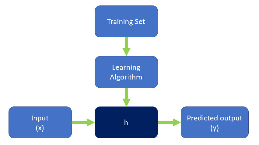
When y is a continuous value, such as a house price or a stock price, this is a regression problem.
When y is only a small number of fixed values (true/false - yes/no), this is a classification problem.
2. Cost Function
We “measure” the accuracy of the hypothesis function using a function. That function is called the cost function.
Before putting down any formula or function, come dig with me through a messy pile of knowledge that I’m sure will help you grasp the core of the
Cost Function.
2.1. The math
2.1.1. Probability and Statistic
In probability and statistics there is a concept called Gaussian Distributed.
That’s right, you’re not misreading.
Gaussianis also a famous feature of…Photoshop, where it blurs the selected area. That feature is calledGaussian Blur.
In probability theory, the normal distribution, also called the Gauss distribution, Gaussian distribution or Laplace-Gauss distribution, is a form of continuous probability distribution (Continuous probability distribution).
The reason I bring up the normal distribution is that by the central limit theorem (Central limit theorem), in the most general form of the normal distribution, the distribution of the sum of very many independent random variables is approximately normal.
That is, the more training examples there are, the closer each training example‘s value is to our hypothesis function.
In short, we pick the parameters so that the distance from the hypothesis function’s graph to the y of the training examples is as short as possible.
2.1.2. Variance
In probability theory and statistics, the variance of a random variable is a measure of that variable’s statistical dispersion; it says how far the variable’s values typically lie from the expected value.
By this definition of variance, the graph representing the expected values is exactly our hypothesis function’s graph. The variance is exactly the value we want as small as possible
The variance of a random variable is the square of the standard deviation.
As said in the previous section, when our set of training example input values is large enough, we can treat each training example as a random variable with a normal distribution.
So we have:
The expected set = hypothesis
$h_\theta(x)=\theta_0+\theta_1x$
The standard deviation:
$latex h_\theta(x^{(i)})-y^{(i)}$
Variance = (standard deviation)2
So the variance over the set of training examples is:
$latex \frac{1}{m}\sum_{i=1}^m(h_\theta(x^{(i)})-y^{(i)})^2$
Our job is to find the minimum value of the formula above.
2.2. Derivative
To find the maximum / minimum value of a function we can use the derivative.
2.2.1. A mathematical example
A ball is thrown into the air. The ball’s height above the ground at any time t is given by the formula:
h = 3 + 14t -5t2
So what is the ball’s maximum height?
Applying the derivative, we solve this problem as follows:
$latex \frac{\text{d}}{\text{d}t}h=0+14-5(2t)=14-10t$
The function above represents the rate of change of the height h at time t. So at the maximum height, the rate of change of the height h = 0 (because the ball stops rising and starts falling).
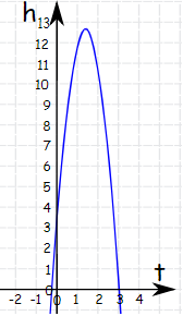
So we have:
[code lang=text] 14-10t = 0
=> t = 1.4 [/code]
So the maximum height is
[code lang=text] h = 3 + 14x1.4 - 10x1.4x1.4 = 12.8 [/code]
2.2.2. Maximum or minimum
How do we know whether a function has a maximum or a minimum value? Going by the graph would take a lot of time and effort.
Here we use the derivative again (one more time):
[code lang=text] f’(t) = 14 - 10t, at t = 1.4 f’(t) = 0
=> f’’(t) = -10, at t = 1.4 f’’(t) = -10 [/code]
This is called the Second Derivative Test, stated as:
When a function’s rate of change = 0 at a point x, then the value of that function’s second derivative at x, if:
Less than 0: that is a maximum value.
Greater than 0: that is a minimum value.
Equal to 0: the function’s maximum/minimum cannot be determined yet.
2.3. The formula
Applying both the derivative and the math above, we get:
$latex \frac{1}{2m}\sum_{i=1}^m(h_\theta(x^{(i)})-y^{(i)})^2$
with
$latex h_\theta(x^{(i)}) = \theta_{0} + \theta_{1}x^{(i)}$
The reason for the 2 in the denominator is to cancel out when we take the derivative. Overall it doesn’t affect the result, since the goal is finding the minimum of the function above.
So we look for the values of $latex \theta_{0}$ and $latex \theta_{1}$ that make the function above smallest.